The Function Representation

In this notebook, we showcase how the function representation of a set of values pre-calculated on a grid is used in lcm, and how it works. Before we dive into the details, let us consider what it does on a high level.

Motivation¶

Consider the last period of a finite dynamic programming problem. The value function array for this period corresponds to the solution of a classic static utility maximization problem. That is, it is the maximum of concurrent utility in each state, where the maximum is taken over actions.

If the state-space is discretized into states $(x_1, \ldots, x_p)$ , the value function array (in the last period) $V^\text{arr}_T$ is a $p$ -dimensional array, where the $i$ -th entry $V^\text{arr}_{T, i} = V^\text{arr}_T(x_i)$ is the maximal utility the agent can achieve in state $x_i$ .

Consider now the Bellman equation for the second-to last period:

V_{T-1}(x) = \max_{a} \left\{u(x, a) + \mathbb{E}_{T-1}\left[V_T(x') \mid x, a\right] \right\},

(1)

where $a$ denotes the action, and $x', x$ denote the next and current state, respectively.

For most solution algorithms, we will need to evaluate the function $V_T$ at a different set of points than the pre-calculated grid points in $V^\text{arr}_T$ .

Ideally, we would like to have a function in the code that we can treat like $V_T$ is written in the equation above: a function that can be evaluated at any valid state $x$ , ignoring the discretization in $V^\text{arr}_T$ . This is precisely what the function representation does.

General Steps¶

To get a function representation of pre-calculated values on a grid (i.e. an array) we need to take care of the following things:

The function will be called with named arguments. Hence, we need to know which argument name corresponds to which array dimension.
The function will be called with values of each dimension (e.g., health taking on a value of 3). However, array elements are retrieved through indexing (maybe an index of 1 corresponds to a value of 3 for health). Hence. we require a mapping from levels to indices.
Continuous variables will take on values that do not occur in the grid. This requires interpolation of the function values found on that grid.

Combining the above allows us to create a function representation of pre-calculated values on a grid, which behaves like an analytical function.

Example¶

As an example, we use the terminal (retired) regime of a simple two-regime consumption-savings model. This regime has a single continuous state (wealth) and a single continuous action (consumption), making it ideal for demonstrating how the function representation works. We use a coarse linearly-spaced wealth grid (10 points) to clearly show the interpolation behavior (of course, with a CRRA/log utility function, one would usually use a log-spaced grid here).

import jax.numpy as jnp

from lcm import (
    AgeGrid,
    DiscreteGrid,
    LinSpacedGrid,
    Model,
    Regime,
    RegimeTransition,
    categorical,
)
from lcm.typing import ContinuousAction, ContinuousState, DiscreteAction, FloatND


@categorical
class WorkingStatus:
    retired: int
    working: int


@categorical
class RegimeId:
    working: int
    retired: int


def next_regime() -> int:
    return RegimeId.retired


def utility_working(
    consumption: ContinuousAction,
    working: DiscreteAction,
    risk_aversion: float,
    wage: float,
    disutility_of_work: float,
) -> FloatND:
    return (
        consumption ** (1 - risk_aversion) / (1 - risk_aversion)
        - disutility_of_work * jnp.log(wage) * working
    )


def utility_retired(consumption: ContinuousAction, risk_aversion: float) -> FloatND:
    return consumption ** (1 - risk_aversion) / (1 - risk_aversion)


def labor_income(wage: float, working: DiscreteAction) -> FloatND:
    return wage * working


def next_wealth(
    wealth: ContinuousState,
    consumption: ContinuousAction,
    labor_income: FloatND,
    interest_rate: float,
) -> ContinuousState:
    return (1 + interest_rate) * (wealth + labor_income - consumption)


def borrowing_constraint(
    consumption: ContinuousAction, wealth: ContinuousState
) -> FloatND:
    return consumption <= wealth


consumption_grid = LinSpacedGrid(start=1, stop=400, n_points=50)

working_regime = Regime(
    transition=RegimeTransition(next_regime),
    constraints={"borrowing_constraint": borrowing_constraint},
    functions={"utility": utility_working, "labor_income": labor_income},
    actions={
        "working": DiscreteGrid(WorkingStatus),
        "consumption": consumption_grid,
    },
    states={
        "wealth": LinSpacedGrid(start=1, stop=400, n_points=10, transition=next_wealth)
    },
)

retired_regime = Regime(
    transition=None,
    functions={"utility": utility_retired},
    constraints={"borrowing_constraint": borrowing_constraint},
    actions={"consumption": consumption_grid},
    states={"wealth": LinSpacedGrid(start=1, stop=400, n_points=10, transition=None)},
)

model = Model(
    description="Simple two-regime consumption-savings model",
    ages=AgeGrid(start=60, stop=62, step="Y"),
    regimes={
        "working": working_regime,
        "retired": retired_regime,
    },
    regime_id_class=RegimeId,
)

params = {
    "discount_factor": 0.95,
    "risk_aversion": 1.5,
    "wage": 10.0,
    "interest_rate": 0.04,
    "disutility_of_work": 0.1,
}

After creating a model, we can access its internal representation. Each regime is processed into an InternalRegime that contains the materialized JAX grids and compiled functions. We use the terminal retired regime for this demonstration.

internal_regime = model.internal_regimes["retired"]

Last period value function array¶

To compute the value function array in the last period, we first generate the utility and feasibility function that depends only on state and action variables, and then compute the maximum over all feasible actions.

from lcm.Q_and_F import _get_U_and_F

u_and_f = _get_U_and_F(internal_regime.internal_functions)

u_and_f.__signature__

<Signature (consumption: 'ContinuousAction', utility__risk_aversion: 'float', wealth: 'ContinuousState') -> ('FloatND', 'FloatND')>

We can then evaluate u_and_f on scalar values. Notice that in the below example, the action is not feasible since the consumption constraint forbids a consumption level that is larger than wealth.

_u, _f = u_and_f(
    consumption=100.0,
    wealth=50.0,
    utility__risk_aversion=1.5,
)

print(f"Utility: {_u}, feasible: {_f}")

Utility: -0.2, feasible: False

To evaluate u_and_f on the whole state-action-space we need to use lcm.productmap, which allows us to pass in grids for each variable.

internal_regime.grids.keys()

dict_keys(['wealth', 'consumption'])

from lcm.dispatchers import productmap

u_and_f_mapped = productmap(func=u_and_f, variables=("wealth", "consumption"))

u, f = u_and_f_mapped(**internal_regime.grids, utility__risk_aversion=1.5)

print(f"Shape of (wealth, consumption) grids: {u.shape}")

Shape of (wealth, consumption) grids: (10, 50)

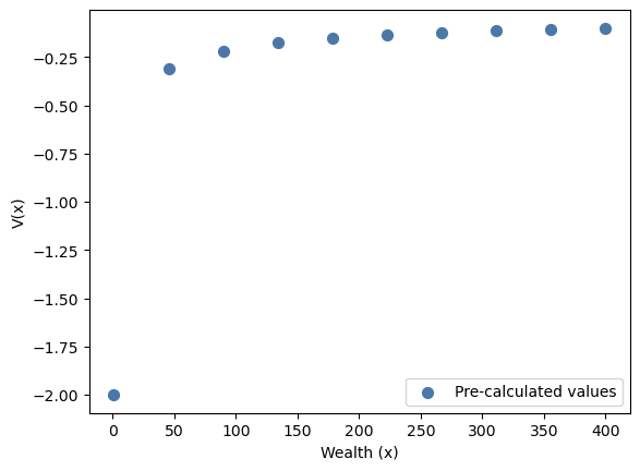
Now we can compute the value function array by taking the maximal utility over all feasible actions (axis 1 corresponds to the consumption dimension).

V_arr = jnp.max(u, axis=1, where=f, initial=-jnp.inf)
V_arr.shape

(10,)

wealth_grid = internal_regime.grids["wealth"]

import matplotlib.pyplot as plt

blue, orange = "#4C78A8", "#F58518"

fig, ax = plt.subplots()
ax.scatter(
    wealth_grid,
    V_arr,
    color=blue,
    s=50,
    label="Pre-calculated values",
    zorder=2,
)
ax.set_xlabel("Wealth (x)")
ax.set_ylabel("V(x)")
ax.legend()
plt.show()

Matplotlib is building the font cache; this may take a moment.

Interpolation¶

What happens now if we want to know the value of $V_T$ at 25 or 75? We need to perform some kind of interpolation. This is where the function representation comes into play, which returns pre-calculated values if evaluated on a grid point, and linearly interpolated values otherwise.

To optimally utilize the structure of the grids when interpolating, the function representation requires information on the state space.

space_info = internal_regime.state_space_info

Setting up the function representation¶

The first step is to generate a function that can interpolate on the value function array. The resulting function can be called with scalar arguments (here this means we can only pass scalar levels of wealth and no grids). It also requires the data on which it interpolates as an argument. The name of this argument can be set using the name_of_values_on_grid argument. Below we use name_of_values_on_grid="V_arr", which implies that the resulting function gets an additional argument V_arr that can be used to pass in the pre-calculated value function array.

from lcm.function_representation import get_value_function_representation

scalar_value_function = get_value_function_representation(
    state_space_info=space_info,
    name_of_values_on_grid="V_arr",
)
scalar_value_function.__signature__

<Signature (V_arr: 'Array', next_wealth: 'Array') -> 'Array'>

We then apply the productmap decorator, which allows us to evaluate the function on a grid of state variables (in this case, just wealth).

value_function = productmap(func=scalar_value_function, variables=("next_wealth",))

Visualizing the results¶

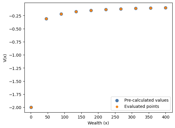
Besides the pre-calculated values at the grid points, we will now add the values generated by evaluating the value function on the original grid points, and on additional points computed by the value function generated by the function representation. We expect the values on the grid points to coincide, and the values on the additional points to be interpolated.

wealth_grid = internal_regime.grids["wealth"]
wealth_points_new = jnp.array([10, 25, 75, 210, 300])

wealth_grid_concatenated = jnp.concatenate([wealth_grid, wealth_points_new])

V_via_func = value_function(next_wealth=wealth_grid_concatenated, V_arr=V_arr)

fig, ax = plt.subplots()
ax.scatter(
    wealth_grid,
    V_arr,
    color=blue,
    s=50,
    label="Pre-calculated values",
    zorder=2,
)
ax.scatter(
    wealth_grid_concatenated,
    V_via_func,
    color=orange,
    s=25,
    label="Evaluated points",
    zorder=3,
)
ax.set_xlabel("Wealth (x)")
ax.set_ylabel("V(x)")
ax.legend()
plt.show()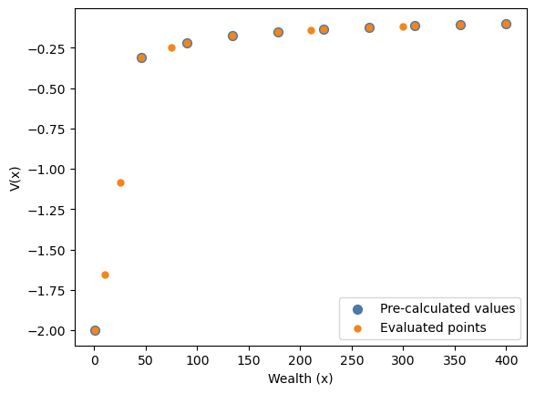

If we now connect the pre-calculated values at the grid points using a line, that is, we perform a linear interpolation on the value function array. We see that the values generated by the function representation lie on that linear interpolation line.

That means, the function representation can simply be thought of as a function that behaves like an analytical function corresponding to this linear interpolation.

fig, ax = plt.subplots()
ax.scatter(
    wealth_grid,
    V_arr,
    color=blue,
    s=50,
    label="Pre-calculated values",
    zorder=2,
)
ax.plot(
    wealth_grid,
    V_arr,
    color=blue,
    label="Linear interpolation",
    zorder=1,
)
ax.scatter(
    wealth_grid_concatenated,
    V_via_func,
    color=orange,
    s=25,
    label="Evaluated points",
    zorder=3,
)
ax.set_xlabel("Wealth (x)")
ax.set_ylabel("V(x)")
ax.legend()
plt.show()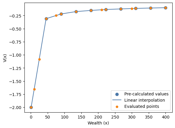

Technical Details¶

In the following, we will discuss the building blocks that are used to implement the function representation.

Label Translator¶

The label translator is used to map the labels of dense discrete grids to their corresponding index in the grid. Currently, PyLCM works under the assumption that internal discrete grids always correspond to their indices. That is, a grid like [2, 3] is not allowed, but would have to be represented as [0, 1] to be valid.

PyLCM converts discrete grids into an internal grid that is directly usable as an index. Thus, the label translator simply is the identity function.

from lcm.function_representation import _get_label_translator

translator = _get_label_translator(in_name="health")
translator.__signature__

<Signature (health: 'Array') -> 'Array'>

translator(health=3)

3

Lookup Function¶

The lookup function emulates indexing into an array via named axes.

Note. These helper functions are important because we use dags.concatenate_functions to combine all auxiliary functions to get the final function representation.

# We want a function that allows us to perform a lookup like this:
V_arr[jnp.array([0, 2, 5])]

Array([-2. , -0.22028813, -0.13457806], dtype=float32)

from lcm.function_representation import _get_lookup_function

lookup = _get_lookup_function(array_name="V_arr", axis_names=["wealth_index"])
lookup.__signature__

<Signature (wealth_index: 'Array', V_arr: 'Array') -> 'Array'>

lookup(wealth_index=jnp.array([0, 2, 5]), V_arr=V_arr)

Array([-2. , -0.22028813, -0.13457806], dtype=float32)

Coordinate Finder¶

For continuous grids (linearly and logarithmically spaced), the coordinate finder returns the general index corresponding to the given value. As an example, consider a linearly spaced grid [1, 2, 3]. The general coordinate value given the value 1.5 is, in this case, 0.5, because 1.5 is exactly in the middle between 1 (index = 0) and 2 (index = 1). The output of the coordinate finder can then be used by jax.scipy.ndimage.map_coordinates for the interpolation.

wealth_gridspec = LinSpacedGrid(start=1, stop=400, n_points=10)

wealth_gridspec.to_jax()

Array([  1.      ,  45.333336,  89.66667 , 134.      , 178.33334 ,
       222.66667 , 267.      , 311.33334 , 355.6667  , 400.      ],      dtype=float32)

from lcm.function_representation import _get_coordinate_finder

wealth_coordinate_finder = _get_coordinate_finder(
    in_name="wealth",
    grid=wealth_gridspec,
)
wealth_coordinate_finder.__signature__

<Signature (wealth: 'Array') -> 'Array'>

To showcase the behavior of the coordinate finder, and how the general indices work, consider the following wealth values:

1: This value is the first value in the original grid, therefore the index must correspond to 0
(1 + 45.333336) / 2: This value is exactly in the middle between the first and second value in grid, therefore the general index corresponds (0 + 1) / 2 = 0.5
395: This value is very close to the last index in the original grid, so the general index will be very close to 9.

wealth_values = jnp.array([1, (1 + 45.333336) / 2, 390])

wealth_coordinate_finder(wealth=wealth_values)

Array([0. , 0.50000006, 8.774436 ], dtype=float32)

Interpolator¶

from lcm.function_representation import _get_interpolator

value_function_interpolator = _get_interpolator(
    name_of_values_on_grid="V_arr",
    axis_names=["wealth_index"],
)

value_function_interpolator.__signature__

<Signature (V_arr: 'Array', wealth_index: 'Array') -> 'Array'>

wealth_indices = wealth_coordinate_finder(wealth=wealth_values)

V_interpolations = value_function_interpolator(
    wealth_index=wealth_indices,
    V_arr=V_arr,
)
V_interpolations

Array([-2. , -1.1548308 , -0.10151813], dtype=float32)

fig, ax = plt.subplots()
ax.scatter(
    wealth_gridspec.to_jax(),
    V_arr,
    color=blue,
    s=50,
    label="Pre-calculated values",
    zorder=2,
)
ax.scatter(
    wealth_values,
    V_interpolations,
    color=orange,
    s=25,
    label="Evaluated points",
    zorder=3,
)
ax.set_xlabel("Wealth (x)")
ax.set_ylabel("V(x)")
ax.legend()
plt.show()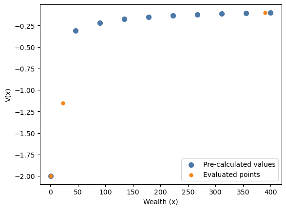

Re-implementation of the function representation given the example model¶

Next, we will outline and implement the steps to re-implement the function representation for the example model specified above. This is intended to help with understanding how the internals of the function representation work.

The Steps¶

We start by listing the required steps. The general idea is to generate functions for the array lookup, interpolation, and so on, with the correct signature signaling their dependence structure. These can then be combined into a single function that performs all necessary steps using dags.concatenate_functions.

Add functions to look up positions of discrete state variables given their labels
In the above example model there are no discrete state variables, so we can skip this step. If there are discrete variables, the lookup functions will coincide with the identity function, as the variables themselves are indices.
Create the lookup function for the discrete part
In this step, a function is generated that allows one to index into the pre-calculated value function array using the labels of the discrete state variables. In the above example model, there are no discrete state variables, so this function returns the value function array untouched.
Create interpolation functions for the continuous state variables
If the model contains (dense) continuous state variables, interpolation functions are required.
1. Add a coordinate finder for each continuous state variable
  This allows us to map values of the continuous variable into their corresponding (general) indices, as required by the interpolator.
2. Add an interpolator
  The interpolator uses the general indices from the last step, to interpolate on the values of the state variable at the corresponding grid points.
Throwing everything into dags

The last step is to throw everything into dags.concatenate_functions. The resulting function is a value function that behaves like an analytical function.

The Implementation¶

# Create the functions dictionary that will be passed to `dags.concatenate_functions`
funcs = {}


# Step 1: Since there are no discrete state variables, we do not require any label
# translator
space_info.discrete_states

mappingproxy({})

# Step 2: Since there are no discrete state variables in the model, the discrete
# lookup coincides with the identity function. Since there are continuous state
# variables in the model, we must interpolate and the data that is returned here is
# used as interpolation data.


def discrete_lookup(V_arr):
    return V_arr


# if there was no interpolation, the entry in the funcs dictionary would have to be
# '__fval__'.
funcs["__interpolation_data__"] = discrete_lookup

# Step 3: (1) First we need to add a coordinate finder for the wealth state variable
from lcm.grid_helpers import get_linspace_coordinate


def wealth_coordinate_finder(wealth):
    return get_linspace_coordinate(
        value=wealth,
        start=1,
        stop=400,
        n_points=10,
    )


funcs["__wealth_coord__"] = wealth_coordinate_finder

# Step 3: (2) And second, we need to add an interpolator for the value function that
# uses the wealth coordinate finder as an input.

from lcm.ndimage import map_coordinates


def interpolator(__interpolation_data__, __wealth_coord__):
    coordinates = jnp.array([__wealth_coord__])
    return map_coordinates(
        input=__interpolation_data__,
        coordinates=coordinates,
    )


funcs["__fval__"] = interpolator

# Step 4: Throwing everything into dags
from dags import concatenate_functions

value_function = concatenate_functions(
    functions=funcs,
    targets="__fval__",
)
value_function.__signature__

<Signature (V_arr, wealth)>

V_evaluated = value_function(wealth=wealth_gridspec.to_jax(), V_arr=V_arr)

fig, ax = plt.subplots()
ax.scatter(
    wealth_gridspec.to_jax(),
    V_arr,
    color=blue,
    s=50,
    label="Pre-calculated values",
    zorder=2,
)
ax.scatter(
    wealth_gridspec.to_jax(),
    V_evaluated,
    color=orange,
    s=25,
    label="Evaluated points",
    zorder=3,
)
ax.set_xlabel("Wealth (x)")
ax.set_ylabel("V(x)")
ax.legend()
plt.show()